The New Technology Characteristic
|
The patented US (7,529,404) hardware based Tunable Filter includes low count electronic components (above), providing much less weight and power to be installed on satellites. This technology in Remote Sensing may include Instruments in electromagnetic radiation in the microwave, infrared, visible, ultraviolet, x-ray, and gamma-ray regimes.
The technology presented is a ground breaking new method for Digital Signal Processing (DSP) purposes, towards providing DOD, DHS, NASA and commercial institutions a tool for detection and identification, with much clarity to resolve false alarms, contrasts and avoid starlight suppression. This simple scheme of detection and identification is posed to open a new window of discoveries to replace the present software based technology.
|
|
Resolution
|
Identification (Resolution) Theory
The newly patented hardware-based, Digital Tunable Filter (7,529,404) shown below (Figure 1), is posed to achieve NASA’s aim in exploration of outer space stars and finding an Earth-like planet much quicker and with far less cost. The operation of the Digital Tunable Filter is very similar to our daily life of watching T.V. It behaves the same way as our brain identification of targets. When we watch T.V. our eyes detects primary colors of a pixel (or group of pixels) and our brain compares the detected colors to a pre-recorded colors (in the brain), on the basis of association. The exception is that the technology does not to pre-load trillions of different shades of color. There are no computation for filtering and identification. Future Advancements The power behind differentiations of colors is based upon probability theory. When we throw a dice, the probability of getting any number (1 to 6) is 1/6. For three dices, the probability is 1/6^3 = 1/216. The same methodology applies for greater resolutions in which the number of dices is represented by number of channels (or primes) and the number of dots on a face of the dice is represented by number of bits of the A/D converter. Thus the number of shades of color of a single pixel (resolutions in visible light) is given by: |
|
- Probability of Detection of shade of color o a pixel = 1/d^p. Equation 1
- Probability of identification with ‘n’ number of pixels = [1/d^p]^n. Equation 2
[1/256^3] ^2 = 1/256^6 = 1/281,474,976,710,656. = 2.81* 10^14.
With four primes and 9 bits of the A/D converter, the odds are 1/ 512 ^4 = 1/ 68,719,476,736. This is 4,096 times more power of resolution. For four primes and 12 bits of the A/D converter, the resolution is 1/281,474,976,710,656 or 16,777,216 times more power of resolution compared to the three primes and 8 bit A/D converter. For two or more pixels the resolution increases exponentially to much greater odds (equation 2).
Note: The above detection Figures of a star by the simulator, is based on 3 primes and 8 bit per prime.
The Achievable four primes and 12 bit per prime provides brightness resolutions of magnitudes of 10^14 better than 10^10 desired by NASA. This technology provides 10^4 or 10,000 time better differentiations in brightness. To separate planets from stars, the combinations of visible light and IR should provide the masking (filter) that is required to detect an Earth like planet surrounded by water. The IR signature of H2O is quite distinct. For a four channel of IR and 12 bits per A/D converter, the equation for resolutions is:
- Probability of Detection = (1/d^p). (1/d^c). Equation 3
This provides resolutions of 1/281,474,976,710,656 * 281,474,976,710,656 = 1/ 2.8 * 10^28.
For two or more pixels the resolution increases exponentially to much greater odds given by.
- Probability of Detection = [1/d^p). (1/d^c)]^n. Equation 4
This technology is posed to resolve the masking and starlight suppression problems economically in shorter time.
Differences in Resolutions Compared with Current DSP Methods
The proposed technology of pixel by pixel filtering is new thus it is hard to find literature to compare the new methodology of filtering and identification to the ongoing methods. Without resorting to a high level of technical comparisons of this Tunable Filter methodology and the present DSP practices (in which itself is a big task).
The advantages of the proposed is best exhibited by the examining and comparing the results of the its simulation (Given Figures).
The present tech Kalman filters, correlation filters and Fast Fourier Transforms (FFT) are currently used to filter and isolate a target from surrounding noise [4, 5]. They have widespread use in pattern recognition, class or cluster recognition in which variety of attributes of a moving object is used for identification and tracking. The filtering and detection is on the cluster bases [13] or motion attributes like velocity [12] or accelerations.
Filter Bandwidth Settings
- The bandwidth can be any band of frequencies or a group of different (not adjacent) bands. It encompasses from the lowest narrowband, which is a single pixel to broadband frequencies for many pixels.
- There is no limitation to the spectral frequencies spacing. Any frequency can be detected as long as their intensity values are pre-loaded in the filter memory.
- For scientific instrumentation, unlike the human retina’s non linarites, the detection can be as linear (flat) as one might expect it to be. Any band of electromagnetic signals either continuous or disjoint is detected.
Speed
The proposed technology provides filtering without calculations. It sets upper and lower received intensities for each prime or IR and if all the primes are detected within the set values, it declares that a pixel is detected. This is done in digital hardware with no equation solving for detection of a target. Because of this, detection starts from the time that all the primary values are available to the filter plus 20 nanoseconds that is the propagation delays of the electronic components. Timing analysis of the proposed hardware based Tunable Filter (Figure 1) indicates filtering speeds of 80 milliseconds for a frame (or picture) of 4,000,000 pixels. This is a breakthrough processing times, to detect hundreds of targets compared to the present DSP practices. This feature should be one of the NASA’s objectives for robotic programs and discoveries of outer space targets.
Differences in Speed compared with present DSP Practices
The current concepts of FFT and Kalman filters extensively use multiplication and addition in either software or hardware to perform detection and thus long delays. As explained above their resolution is rather poor. Lack of resolutions in detection, most often forces the sensor platform to send raw data to a “center” for post processing and decision making. The delays due to the pre and post processing of data are a hindrance to real time immediate operations.
The results extended studies of the present methodology with respect to speeds are outlined below:
- Kalman filtering is probably the most commonly used algorithm for implementing the tracker, although recently Condensation algorithm [7] and mean shift algorithm [4] have shown to provide certain advantages especially in the presence of significant background clutter. The Kalman filter is primarily used for identification and tracking slow moving targets [11, 12, and 13]. Tracking is enhanced by the structural information perceived from the moving objects, which improves the classification [13]. Tracking is initiated every time a new moving object is determined in the scene and the features found to fulfill the predefined criteria [13].
- Kalman filter is considered to be too computationally infeasible for image super-resolution due to the size of the images and thus the state space involved [9]. It is assumed that a person changes its walking direction and walking speed according to Gaussian distributions, thereby, the translational velocity is assumed to lie between 0 and 150 cm/s.
- Variations of this filter have a widespread use in detections of moving cars in a parking lot, but they are not suited to track and count vehicles in a fast moving street or highway [12]. Tracking non-rigid targets in low-resolution images has long been realized as a region based correspondence problem, in which each target is mapped from one frame to the next according to its position, dimension, color and other contextual information. When multiple targets exist and their dimensions are not negligible in comparison with their velocities, occlusion or grouping of these targets is a routine event. This brings about uncertainty for the tracking, because the contextual information is only available for the group and individual targets cannot be identified. [10] [14].
Calibration
New Methodology in Calibration of Channels
The technology (US 8159568 Ned M. Ahdoot) uses two methods of calibration. The first method is to calibrate based upon the calibration channel such as gray scale in visible light or by adding one or more calibration channels for IR systems. The second method is to calibrate the data channels based upon the availability of the adverse condition degree (data) that affect regular data channels. In the first method, the received data from calibrating channels are compared to known (ideal) value and calibration factors are generated to calibrate the regular data channel.
Eight channel calibration and filtering
Figure 3 is the block diagram is the hardware implementation for calibration of data channels due to adverse environmental conditions and filtering. The channels are previously undergone radiometric correction for system imperfections (Fig. 5 below), and then they are calibrated before filtering. An environmental factor calibration (normalization, attenuation) for each channel is based upon comparing a set of wavelengths calibration intensities (21, 31, 32 and 33), that are added for calibrating data channels that are received in adverse environmental conditions. These calibration channels are compared with a known intensity magnitude received in an ideal environment condition. The result of comparison provides a calibration factor to calibrate normal channels. Calibration factors are generated either for a specific data channel or a group of data channels (21, 31, 32 and 33); with the ability of cascading several calibration channels to arrive at the final calibration factor to be shared (inhibit Figure 3A) to have a choice of calibrate or not calibrate any data channel.
Figure 3 Block 10 is a Calibration Function Generator Memory, in which it receives the calibration intensity from calibration sensor and generates a calibration factor (25). This calibration factor is sent to the Calibration Memories 11, and 14, that receives the regular data channel and calibrates it with the calibration factor. Block 16 is a cascaded Calibration Factor Generator shown in Figure 3A and to calibrate regular data channels.
The generated function is amended to the received channel data intensity (24, and 26) and the combination is used as an address to Calibration Memories (11 and 14). The data within the Calibration Memories are pre-loaded during the initialization, in which the calibration factor is the most significant bits that points to a set of calibrated data addressed by the received channel data.
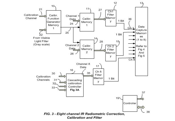
Table 1 below, shows the calibration data intensity, and the corresponding pre-loaded normalization factor. The pre-loaded normalization factors are the result of solving equations of calibrations or empirical values to calibrate data channels in real time. Normalization factor lines of data are amended to the detected intensity of regular data channel to address Calibration Memory (block 11) for calibration (in this case multiplication). Blocks 12, 15 and 17 acts like the calibration memories in Figure 1 and if all the eight channel intensities fall within specified limits (Tunable Filter of visible light Figure 1 above) and receiving a “1” from all filter memories of Blocks 12, 15 and 17 a match (and gate) is decoded by block 13 for detection of an element In all IR channels.
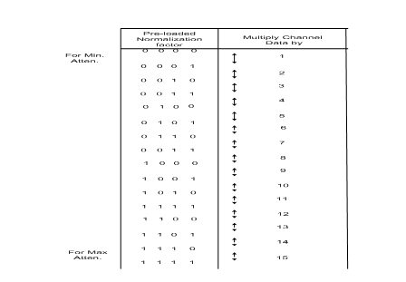
Table 1 – Calibration function generation pre-stored in the memory
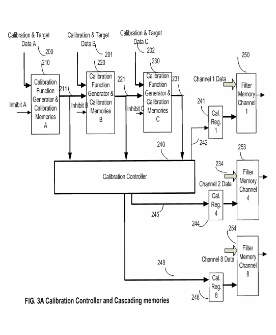
Figure 3A Calibration Controller and Cascading Memories
In the second method the technology allows for calibration due to different variables that are related to the adverse environments conditions (such as lighting, smog, rain, etc.,) that affect the data known, measured intensities of, adverse environmental conditions like rain, humidity, brightness, etc. are used to retrieve a pre-loaded calibration factor from memory to calibrate the regular data channel sequentially (Figure 4 below). For both methods calibration takes place continuously within pixel timing periods (Estimated times of 50 to 70 nanoseconds time limits per channel and one environmental variable). The above methods are the result of the awarded patent for calibration and measurement of various gases remotely. Refer to Hardware implemented pixel level digital filter and processing of electromagnetic signals. Apr, 17, 2012: US 8159568 Ned M Ahdoot:
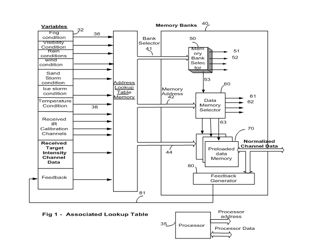
Figure 4: Memory based hardware (sequencing) to calibrate Visible light and IR channels (For myriad of conditions under which target detection must be accomplished.)
Continuous Calibration
The new calibration methods use memories to avoid time consuming calculations of calibration. Detected strengths of data signals in their respective bands are compared to the known values (first method) and the results are used to normalize regular data channels accordingly eliminating calculations. Calibration takes place continuously on 50 to 70 nanoseconds (high speed electronics) time limits for a channel and for a variable. A large density sequencing memory RAM structure (Figure 4 above) is used for calibration. The adverse environments conditions (variable data) are used as an address to the sequencing RAM to fetch previously loaded calibration factors. The calibration factors are derived mathematically or by empirical tests. The recent advancements in memory densities increases allows for high addresses to implement this addressing scheme.
Calibration Methodology
The Figure 3D depicts the percent transmittance of various elements such as H2O, O2, O3, and C02 in 0.4 to 2.5 micrometer spectrum wavelength. H2O and CO2 energy transmittance is zero in wavelengths 1.3 to 1.4, and 1.8 to 1.9 micrometer wavelengths. The element CO2 has the heights transmittance in wavelengths 2.0 to 2.4 micrometers.
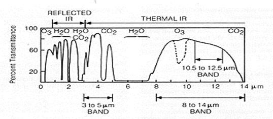
Figure 3D – Channel calibration and filtering spectrum
To accommodate a condition in which multiple environmental adverse conditions may exist, a regular data channel will be calibrated in a Cascading Calibration Scale Generator Memories. Block 16 is a cascaded Calibration Factor Generator to calibrate a regular data channels. More explanation is provided.
Radiometric Corrections due to system imperfections
The radiometric imperfections are system based and they vary from system to system. The imperfections are categorized to affect all pixels or some of the CCD related Pixels. This invention deals with these imperfections individually in a cascading correction memory system that deals with individual imperfections on pixel by pixel level or the imperfections on system level Figure 5 Below. For instance for Focal Point Array (FPA) temperature variations, adjustments are made for all the FPA pixels affected due to temperature variation. These corrections are done automatically regardless of spacecraft location either in a flying mission or in the factory for development. The radiometric imperfections are system based and they vary from system to system. Each system may contain some or all of the following imperfection issues:
- Optical distortions and noises
- Optics (vignetting, shading)
- Defocusing (optics)
- Optical Crosstalk
- Differences in spectral responsivity (spectral balance)
- Flare light (scattering)
- Misalignment of illumination and scan line
- Shading (light drop) at one side of the CCD line
- Different noise patterns between the CCDs used
- ADC quantization noise
- Amplifier noise
- Distortions due to lens or other optics (radial and tangential distortion)
- CCD line imperfections, misalignment and overlap
- CCD Area imperfections
- Grey scale linearity
- Dust
- Electronic noise (dark signal/thermal noise, dark signal no uniformity, photo response, non-uniformity (vertical stripes, gain/offset) electronic cross-talk
- Smear due to movement (linear CCDs)
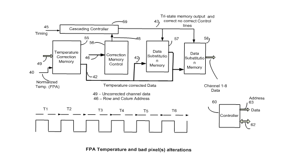
Figure 5 - FPA temperature adjustments and individual pixel(s) modification
Radiometric System induced imperfection Correction
Figure 5 is for the FPA temperature corrections and individual correction for some of the FPA’s bad pixels. Block 55 is for temperature corrections and the rest of the blocks for bad pixels modification. This proposal covers only the FPA temperature adjustments of the received channel intensities.
Block 55 receives pixel data along with normalized temperature of the FPA as an address to the temperature correction memory. The data within this memory is pre-written in which the address containing the sensor pixel data along with the normalized FPA temperature is the corrected data according to the normalized temperatures. Table 2 is a chart showing the address to the memory including normalized temperature and the output data. The normalized temperature is shown as a four (most significant bits) binary numbers wherein each one of the four bits contains 256 memory locations (that are not shown). The memory data for each one of 256 locations are pre-registered (calculated or empirically) to indicate a corrected value. The uncorrected pixel data is shown as eight bit xxxxxxxx. The corrected data in memory) that no corrections are needed. Of course, this is a simplistic example to convey the method.
Referring again to Figure 5, the row and column addresses (46) is input to block 56, corresponding to each pixel is the input to individual bad pixel corrections. The data for this memory is pre-loaded to select an origin of a data and correct no correct information intended for each Cascading Correction Memories, Blocks 57 and 58.
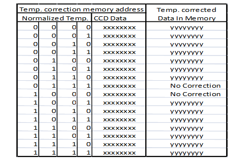
Table 2 Temperature normalization for FPA data correction
The above procedure is suitable for few adjustments due to system imperfections. The same method of channel data adjustments can be used by using the memory based calibration corrections Figure 4. This is not covered in this proposal.
Significance and Conclusion
Implementation of this new technology that will provide a significant breakthrough for the discovery of organic and inorganic compounds with the existing video data From Europa or other outers pace planets resulting in the discovery of Earthlike environments. With its future implementation in hardware, it will drastically cut size, weight and costs of payloads by requiring much smaller optical equipment.
For effective, and low cost system of identification of compounds in Europa, the technology addresses three important aspects of image processing.
1) Provide a high resolution detection capability and minimize false alarms,
2) Provide ability to process data in the least amount time.
3) Provide capability to monitor and quantize compounds and gases even in the presence of other gases.
Higher resolutions will provide capturing of more targets in a single frame of video and differentiation of a target from a noise, (avoiding false alarms). Higher speeds of processing allow receiving, and processing video data from many different sensors (fusion) for shortest possible time.
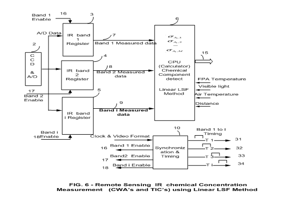
Remote Concentration Measurements
The preferred method for the measurement outlined in the patent is based upon a recent study and recommendation for measurements of chemical agents by, Michael B. Pushkarsky1, Michael E. Webber1, Tyson MacDonald1 and C. Kumar N. Patel and Department of Physics & Astronomy, University of California. Los Angeles, CA 90095.
The above paper for concentration measurements of harmful gases is based upon using laser technology in different frequencies and is based upon a closed environment testing. However, the same concept for utilizing lasers can be used (due to drastic increases in identification (filtering) proposed by this paper) to measure concentrations of substances or gases even in the presence of other gases using a remote technology of visible light and IR.
The UCLA study presents an analytical model for evaluating the suitability of optical absorption based spectroscopic techniques for detection of chemical warfare agents (CWAs) and toxic industrial chemicals (TICs) in a ambient air (closed system in which the sampled contaminated air is introduced to measurement system). The study is based upon sensor performances that are modeled by simulating absorption spectra of a sample containing both the target and multitude of interfering species as well as an appropriate stochastic noise for determining the target concentrations from the simulated spectra via a least square fit (LSF) algorithm. The distribution of the LSF target concentrations determines the sensor sensitivity, probability of false positives (PFP) and probability of false negatives (PFN). Their model was applied to CO2 laser based photoacosutic (L-PAS) CWA sensor and predicted single digit ppb sensitivity with very low PFP rates in the presence of significant amount of interferences. This approach will be useful for assessing sensor performance by developers and users alike; it also provides methodology for inter-comparison of different sensing technologies.
Please refer to the patent April, 17, 2012: US 8159568 Ned M Ahdoot: for measurements of the concentrations of chemicals even in the presence of adverse environment conditions. The technology provides for a detection and measurement system to be deployed on satellites or a high flying plane, for immediate detection and measurements.
For effective, and low cost system of identification of compounds in Europa, the technology addresses three important aspects of image processing.
1) Provide a high resolution detection capability and minimize false alarms,
2) Provide ability to process data in the least amount time.
3) Provide capability to monitor and quantize compounds and gases even in the presence of other gases.
Higher resolutions will provide capturing of more targets in a single frame of video and differentiation of a target from a noise, (avoiding false alarms). Higher speeds of processing allow receiving, and processing video data from many different sensors (fusion) for shortest possible time.
Remote Concentration Measurements
The preferred method for the measurement outlined in the patent is based upon a recent study and recommendation for measurements of chemical agents by, Michael B. Pushkarsky1, Michael E. Webber1, Tyson MacDonald1 and C. Kumar N. Patel and Department of Physics & Astronomy, University of California. Los Angeles, CA 90095.
The above paper for concentration measurements of harmful gases is based upon using laser technology in different frequencies and is based upon a closed environment testing. However, the same concept for utilizing lasers can be used (due to drastic increases in identification (filtering) proposed by this paper) to measure concentrations of substances or gases even in the presence of other gases using a remote technology of visible light and IR.
The UCLA study presents an analytical model for evaluating the suitability of optical absorption based spectroscopic techniques for detection of chemical warfare agents (CWAs) and toxic industrial chemicals (TICs) in a ambient air (closed system in which the sampled contaminated air is introduced to measurement system). The study is based upon sensor performances that are modeled by simulating absorption spectra of a sample containing both the target and multitude of interfering species as well as an appropriate stochastic noise for determining the target concentrations from the simulated spectra via a least square fit (LSF) algorithm. The distribution of the LSF target concentrations determines the sensor sensitivity, probability of false positives (PFP) and probability of false negatives (PFN). Their model was applied to CO2 laser based photoacosutic (L-PAS) CWA sensor and predicted single digit ppb sensitivity with very low PFP rates in the presence of significant amount of interferences. This approach will be useful for assessing sensor performance by developers and users alike; it also provides methodology for inter-comparison of different sensing technologies.
Please refer to the patent April, 17, 2012: US 8159568 Ned M Ahdoot: for measurements of the concentrations of chemicals even in the presence of adverse environment conditions. The technology provides for a detection and measurement system to be deployed on satellites or a high flying plane, for immediate detection and measurements.